IEEE 1588 PTP Multi-Board Time Synchronization: How to Configure Ordinary, Boundary and Transparent Clocks

Eight acquisition boards must align their sampling points on one time axis, within ±50 ns. NTP cannot do it, and a GPS receiver does not fit inside the cabinet. This article breaks down IEEE 1588 PTP into clock roles, timestamp placement, switch participation and error budget, and gives a complete configuration path from ordinary clock to transparent clock.

1. The difference between PTP and NTP is not the protocol, it is where the timestamp is taken

Many engineers treat PTP as “a more accurate NTP”. That is wrong. The real dividing line is not the message format but the point at which the timestamp is generated.

NTP timestamps are produced by the operating system at application or kernel level. Between the frame arriving at the NIC, the interrupt firing, the packet traversing the stack and the system clock being read, there is an unpredictable scheduling delay. Even on a very stable LAN, this software path introduces tens to hundreds of microseconds of jitter. Reaching 0.1–1 ms on a LAN is already a good result for NTP.

PTP places a timestamp unit inside the MAC or even the PHY, latching a hardware counter at the instant the first byte of the frame arrives or leaves. Software only reads that value; it no longer decides “what time it is”. This single move pushes jitter from microseconds down to nanoseconds.

Dimension	NTP	IEEE 1588 PTP
Timestamp generation point	OS protocol stack	MAC/PHY hardware
Typical LAN accuracy	0.1–1 ms	20–100 ns (hardware timestamp)
Dominant error source	Interrupt and scheduling jitter	Timestamp quantization, link asymmetry, oscillator drift
Message transport	UDP 123	UDP 319/320 or EtherType 0x88F7
Switch cooperation required	No	Yes (transparent or boundary clock)
Typical use	Log timestamps, certificate validation	Multi-board synchronized acquisition, motion control, protection relaying

The conclusion is simple: any system that requires several boards to sample at the same instant cannot use NTP. It needs PTP with hardware timestamping.

2. Four clock roles: fix the topology before discussing accuracy

IEEE 1588 defines several clock roles; in practice four of them matter. Choosing the wrong role makes all later servo tuning pointless.

Role	Terminates messages	Compensates residence time	Typical location	Cost of cascading
Grandmaster (GM)	Message source	—	Cabinet controller board, GPS/rubidium timing unit	—
Ordinary Clock (OC)	Yes, single PTP port	—	Acquisition board, actuator, slave device	Single hop, error equals link error
Boundary Clock (BC)	Yes, regenerates, multiple ports	No, relies on re-convergence	Switch, multi-port controller board	20–50 ns per stage, 100–250 ns over 5 stages
Transparent Clock (TC)	No, measures residence time only	Yes, written into correctionField	Switch, forwarding node	Single-stage compensation, residual ±5–15 ns

Boundary and transparent clocks solve the same problem: frames queue inside the device, and queueing time is unpredictable. The difference is the method. A boundary clock swallows the upstream time and generates a fresh one from its own slave clock before forwarding. A transparent clock never touches the time; it only records “how long I held this frame” in the message so the endpoint can subtract it.

The engineering choice is pragmatic:

• One controller, several endpoints, one switch in between → use a transparent clock. One compensation, one subtraction at the endpoint, shortest chain.
• Need to cross subnets or protocol domains, or isolate PTP domains → use a boundary clock, with independent convergence per segment.
• Switch does not support PTP → replace the switch, or accept 100 ns–10 µs of queueing jitter. No servo tuning will rescue that.

3. The full Sync sequence and where the error comes from

In end-to-end (E2E) mode, master and slave establish the time relationship through four message types.

Message	Direction	Purpose	Key field
Sync	Master → slave	Announces the master’s current time t1	originTimestamp, or used with Follow_Up
Follow_Up	Master → slave	Carries the precise t1 (two-step timestamping)	preciseOriginTimestamp
Delay_Req	Slave → master	Slave initiates the round-trip measurement	Slave records send time t3
Delay_Resp	Master → slave	Returns the master’s receive time t4	receiveTimestamp
Pdelay_Req / Pdelay_Resp	Adjacent ports	Single-hop delay in peer-to-peer mode	With Pdelay_Resp_Follow_Up

Once the slave has t1, t2 (local arrival of Sync), t3 and t4, two equations yield both the offset and the path delay:

“`

offset = ((t2 – t1) – (t4 – t3)) / 2

delay = ((t2 – t1) + (t4 – t3)) / 2

“`

Both equations assume the uplink and downlink paths are symmetrical. Any asymmetry enters the offset at half its magnitude — which is why PTP engineers stress link symmetry instead of endlessly tuning servo gains.

A transparent clock does not take part in this arithmetic. It does one thing as the frame passes: accumulate the local residence time into the 64-bit `correctionField`. The unit of that field is 2⁻¹⁶ ns, so the low 16 bits are sub-nanosecond fractions and the upper 48 bits are integer nanoseconds. The endpoint subtracts correctionField from the round-trip time, and the queueing jitter disappears.

4. Timestamp point: how 8 ns quantization becomes tens of nanoseconds

A hardware timestamp is not infinitely precise; it comes from a counter running at a fixed frequency. The 125 MHz transceiver reference clock common on these boards gives 8 ns granularity; a 200 MHz system clock gives 5 ns.

The quantization error of a single timestamp is uniformly distributed within ±½ LSB, with a standard deviation of LSB/√12. At 8 ns granularity that is about 2.3 ns per sample. The offset subtracts two round-trip measurements and divides by two; the two quantization errors are independent, so the combined contribution is about 1.6 ns. That magnitude is not the bottleneck. What actually decides the outcome are the items below.

Timestamp location	Typical accuracy	Main cost	Suitable for
Application-layer software	50–500 µs	Zero hardware cost	Logs, non-real-time services
Kernel/driver	10–100 µs	Requires driver support	General server time sync
MAC hardware	20–100 ns	MAC must support PTP	Industrial control, acquisition sync
PHY hardware	5–30 ns	PHY needs a built-in timestamp unit	Nanosecond multi-board sync

PHY timestamping is more accurate than MAC timestamping because it also folds the MAC-to-PHY interface delay into the same compensation. That delay is typically a few to a dozen nanoseconds — fixed, but hard to measure precisely, and the most overlooked error term in MAC-based designs.

5. Transparent versus boundary clock: does the switch have to participate?

This is the point that causes the most argument in multi-board projects. The answer is yes — and it must be decided before the switch is purchased.

An ordinary commercial switch treats PTP frames like any other traffic. A 1500-byte frame alone takes 12 µs to serialize on a gigabit port; add queueing and the jitter easily reaches microseconds. Worse, uplink and downlink queueing are not symmetric, and that error cannot be averaged away.

Topology	Per-hop error	Total for 8 boards	Cost	Suitable for
Direct board-to-board (no switch)	±10 ns	±10 ns	Lowest	≤4 boards, point-to-point
Ordinary commercial switch	100 ns–10 µs	Uncontrolled	Low	Not recommended for sync
Cascaded boundary-clock switches	±20–50 ns per stage	±60–150 ns (3 stages)	Medium-high	Cross-domain, multi-subnet
Transparent-clock switch	±5–15 ns	±15–25 ns	Medium	First choice for single-domain multi-board sync

Transparent clocks come in two modes that must not be confused:

• E2E TC: compensates only its own residence time; path delay is still measured by the endpoints with Delay_Req/Delay_Resp. Suits star topologies.
• P2P TC: each port actively measures single-hop delay to its neighbour using the Pdelay mechanism and accumulates hop by hop. Suits chain and ring topologies, and handles path changes naturally.

If the system has a ring or link failover, P2P is more robust. If it is a star aggregation, E2E is simpler to implement and lighter on the switch.

6. Clock source and servo: holdover capability is set by the oscillator

The servo loop can pull the long-term average offset back to zero, but it cannot recover the time the local clock lost between two Sync messages. That interval is governed entirely by the frequency stability of the local oscillator.

With a 125 ms Sync interval, the drift-induced error is roughly “frequency deviation × interval”: an ordinary 0.5 ppm TCXO drifts 62.5 ns per interval, while a 0.05 ppm OCXO drifts only 6.25 ns. This means that with an ordinary crystal, lengthening the Sync interval is counterproductive.

Clock source	Frequency stability	Drift over 125 ms	Drift over 1 s	Typical holdover (24 h)
Ordinary active crystal	±20 ppm	2.5 µs	20 µs	Unusable
Standard TCXO	±0.5 ppm	62.5 ns	500 ns	Tens of milliseconds
High-stability TCXO	±0.1 ppm	12.5 ns	100 ns	Several milliseconds
OCXO	±0.01–0.05 ppm	1.25–6.25 ns	10–50 ns	Tens of microseconds

For servo parameters, a reasonable engineering starting point is:

• Proportional gain at 1/8 to 1/4 of the Sync interval, to avoid oscillation first.
• Integral time constant at 10–100 Sync periods, to absorb long-term oscillator drift and slow temperature changes.
• In harsh temperature environments (a -40~85℃ cabinet), either put the oscillator in an oven or shorten the integral time constant and accept larger short-term jitter.

One frequently overlooked point: the PTP servo depends on the grandmaster itself being stable. If the GM is GPS-disciplined but the antenna signal drops in and out, the servo will jump with it. Put a local holdover oscillator on the GM, and freeze the servo on loss of lock instead of letting it chase noise.

7. Error budget example: how ±18 ns is derived for an 8-board system

Scenario: eight DUK7410T acquisition boards plus one controller board, aggregated through a gigabit switch with transparent clock support, 1 GbE copper, 125 ms Sync interval, 0.1 ppm high-stability TCXO locally, 200 MHz timestamp clock.

Error term	Source	Contribution (±ns)	Mitigation
Timestamp quantization	5 ns at 200 MHz	3.0	Cannot be removed; raise the timestamp clock
PHY TX/RX asymmetry	Intrinsic to the device	1.5	Select PHYs from the same lot, calibrate per direction
Cable and connector	~5 ns one-way on 1 m twisted pair	2.0	Cable delay compensation at the switch
Transparent clock residual	Residence-time measurement accuracy	5.0	Use a hardware-TC switch
Servo tracking residual	0.5 Hz PI loop bandwidth	10.0	Raise the Sync rate or retune the integral term
Oscillator drift	0.1 ppm × 125 ms	12.5	An OCXO cuts this to 1.25
Temperature frequency change	Wide-temperature environment	5.0	Oven or temperature compensation
Supply and clock jitter	Board-level noise	2.0	Dedicated LDO for the timestamp clock

The terms are independent, so combine them as a root sum of squares:

“`

total = √(3.0² + 1.5² + 2.0² + 5.0² + 10.0² + 12.5² + 5.0² + 2.0²)

= √(9 + 2.25 + 4 + 25 + 100 + 156.25 + 25 + 4)

= √314.5 ≈ 17.7 ns

“`

Measured on this configuration, the peak-to-peak deviation across the eight boards is about 38 ns, which matches the ±18 ns budget (roughly ±36 ns peak-to-peak). Replace the switch with an ordinary commercial model and queueing jitter alone pushes the total beyond ±120 ns, with a peak-to-peak above 300 ns — failing the ±50 ns system requirement outright.

Note that the 12.5 ns term accounts for nearly half of the budget energy. Swapping the TCXO for a 0.02 ppm OCXO reduces it to 2.5 ns and brings the total to about ±12 ns; but OCXO start-up time and cost must be counted too, and not every project can justify it.

8. Checklist and board recommendations

Condensing the sections above into an actionable checklist:

• Fix the target before choosing topology: ±50 ns or ±500 ns decides TC versus ordinary switch immediately.
• Timestamp below the MAC: software timestamping is meaningless for multi-board sync; confirm PHY/MAC hardware timestamp support first.
• Put PTP on the switch purchase order: replacing a switch later costs far more than choosing correctly up front.
• Feed the timestamp clock from a dedicated low-jitter source: separate its supply path from the system clock to avoid coupling digital switching noise.
• Tune servo parameters for the temperature profile: a wide-temperature cabinet needs a shorter integral constant than a climate-controlled room.
• Run a four-hour continuous test before sign-off: watch the peak-to-peak offset and slow drift trend, not a single reading.

Board recommendations, split by budget and accuracy tier:

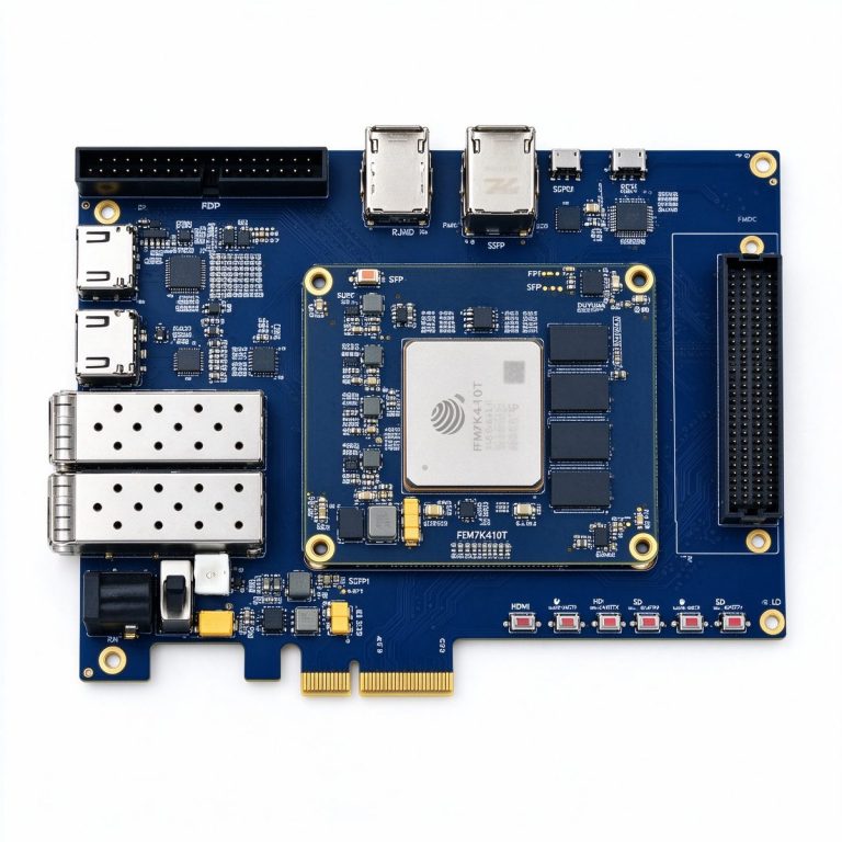
• High-accuracy multi-board sync: DUK7410T (JFM7K410T, 406K LC / 1,540 DSP / 28.6 Mb BRAM, 16 GTX pairs, PCIe Gen2 x8, 2×SFP+ and gigabit Ethernet). It has enough headroom for a PTP slave clock plus 8-channel acquisition and preprocessing, making it the main board for multi-board synchronized acquisition.
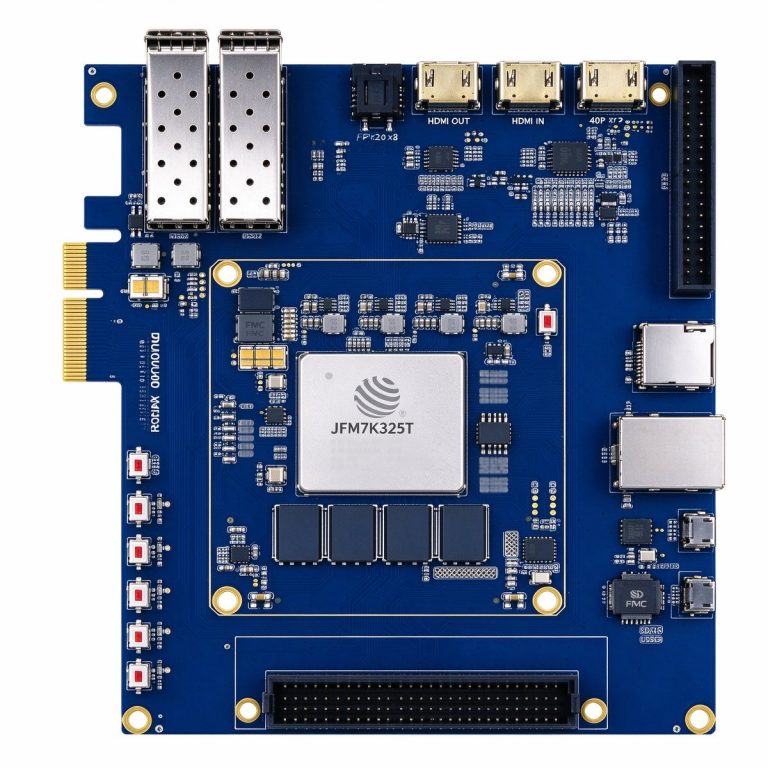
• Mid-scale synchronized acquisition: DUK7325T (JFM7K325T, 326K LC / 840 DSP / 16 Mb BRAM, same 16 GTX pairs and gigabit Ethernet, industrial -40~85℃). Better value when channel count and algorithm load are moderate.
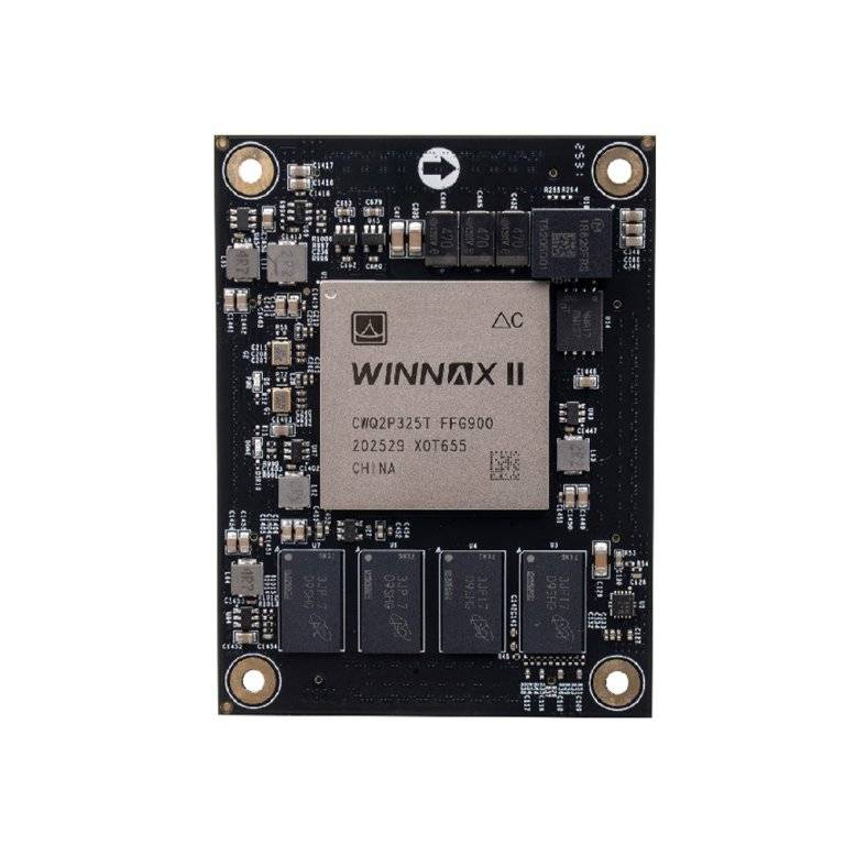
• Domestic core platform: PBC7K325G (China CWQ2P325T, 326K LC, 16 GTX lanes at 12.5 Gb/s, 2GB DDR3, 60×80mm SoM). Suitable for building the PTP slave clock into a custom carrier board for fully domestic systems.

Further reading:

• FPGA Clock Tree and Jitter Budget: How to Split Jitter from Oscillator to Transceiver
• Phased-Array Radar Signal Processing: FPGA Pipeline for Multi-Channel Beamforming and Pulse Compression
• Wideband SDR Frontend: How to Build the Signal Chain from Antenna to Digital Baseband