Phased-Array Radar Signal Processing: Multi-Channel Beamforming and Pulse Compression on an FPGA Pipeline
A phased-array radar points at targets electronically, with no moving parts. The real compute burden is not the antenna but the backend: every echo channel must run digital beamforming, pulse compression and target detection simultaneously. This article breaks that pipeline into calculable data rates and resource budgets, and shows how to build it on FPGA boards.
Why phased arrays need FPGA
A traditional mechanically scanned radar looks one way at a time, so the backend only handles one signal path. A phased array has N antenna elements, each with its own T/R module and ADC. N echo streams must enter the digital domain at the same time to form beams digitally (DBF).
That creates two hard constraints:
- Very high data rate: N ADC channels sample in parallel; the larger N and the faster the sampling, the more bandwidth the backend needs;
- Extremely low latency: beamforming and pulse compression are pipeline-style — you cannot batch and compute; the array must finish processing within each pulse period, or the next pulse arrives.
CPU and GPU cannot deliver this “multi-channel parallel + microsecond pipeline” determinism — that is exactly where FPGA sits.
The complete radar signal processing pipeline
A typical digital phased-array backend, from ADC to target plot, is a pipeline like this:
1. Multi-channel ADC capture: one channel per element, 12–16 bit, sampling from tens to hundreds of MSPS;
2. DDC digital down-conversion: per-channel mixing + low-pass filter + decimation to baseband complex (I/Q);
3. DBF digital beamforming: N baseband streams are complex-weighted and summed per target direction;
4. Pulse compression (matched filter): matched-filter the LFM (chirp) signal to compress a wide pulse into a narrow one, improving range resolution;
5. CFAR constant false-alarm detection: detect targets on compressed data and suppress clutter;
6. Plot extraction and reporting: package detected range/angle/amplitude and send to host.
FPGA fits steps 2–5 into one clock domain, running the whole chain within each pulse period (tens to hundreds of microseconds).
The data-rate math
Take a 16-channel array at 125 MSPS, 14 bit per channel:
| Stage | Formula | Result |
|---|---|---|
| Single-channel raw rate | 125 MSPS × 14 bit | 1.75 Gbps ≈ 218 MB/s |
| 16-channel total rate | 16 × 1.75 Gbps | 28 Gbps ≈ 3.5 GB/s |
| DDC baseband complex rate | 16 ch × 125 MSPS × (16 bit I + 16 bit Q) | 8 Gbps ≈ 1 GB/s |
| DBF complex MAC throughput | 16 ch × 125 M samples/s × 1 complex mul | 2 G complex MAC/s |
| 4096-point pulse-compression FFT | 125 MSPS ÷ 4096 | ≈ 30 FFTs per channel per second |
The key number: 16 parallel channels, 3.5 GB/s raw data into the backend. JESD204B/C high-speed serial links are built for exactly this — each ADC uses one serial lane instead of a wide parallel bus.
What DBF and pulse compression each consume
Digital beamforming (DBF)
DBF is essentially: N complex streams, each multiplied by a complex weight w(n), then summed.
- Every sample point needs N complex multiplications (4 real muls + 2 adds);
- With N=16, 16 complex muls run in parallel each clock — FPGA DSP blocks are naturally parallel;
- Weights w(n) are computed from target steering angle (w(n)=e^(-j·2π·n·d·sinθ/λ)) and stored as lookup tables.
FPGA runs DBF with essentially zero instruction overhead — just fill the DSP blocks with parallel multiply-accumulate.
Pulse compression (matched filter)
The standard LFM pulse compression is the “frequency-domain method”: input FFT × matched filter coefficients → IFFT.
- 4096-point FFT, one per channel;
- FPGA has built-in streaming FFT IP, fixed microsecond latency;
- 16 channels can time-share one FFT core, or run 16 in parallel.
A 4096-point single-precision FFT uses a few hundred DSP blocks and a few Mbit BRAM — easily fits on a board like XCKU15P.
Three board tiers
Different channel counts and update rates need different FPGA resources:
| Board | FPGA platform | Radar scale | Why |
|---|---|---|---|
| XCKU15P core board | Kintex UltraScale+ | 16–64 channel, high-update-rate short-range radar | Abundant logic, GTH transceivers for multiple JESD204B/C lanes, enough DSP for parallel DBF + multi-channel FFT |
| DUF7690T | FudanMicro JFM7VX690T (pin-compatible with XC7VX690T) | Domestic high-reliability radar node | Virtex-7 class, industrial temperature, for supply-chain and reliability-sensitive automotive/security radar |
| DUK7410T | FudanMicro JFM7K410T (pin-compatible with XC7K410T) | 4–8 channel, low-cost prototyping | Kintex-7 class, lower cost; enough for small-array DBF and single-channel pulse compression, for algorithm validation and low-volume production |
A typical split: algorithm teams use DUK7410T for 4-channel waveform and detection prototyping, then port to DUF7690T for domestic production, or move up to XCKU15P for larger-array engineering units.
Case: 16-channel short-range security radar
A short-range security radar used a 16-element line array at 10 GHz, 100 MHz bandwidth, 5 kHz PRF:
- 16 ADC channels feed FPGA over JESD204B;
- DDC drops each channel to 10 MHz complex baseband;
- DBF forms 4 simultaneous receive beams covering different azimuth angles;
- 4096-point frequency-domain pulse compression shrinks a 20µs pulse to about 5 m range resolution;
- Cell-averaging CFAR outputs target plots over PCIe to host.
Measured: single-pulse processing latency about 80µs, well under the 200µs pulse period; FPGA resource use about 60% (DSP and BRAM).
Phased-array “electronic scanning” sounds like an antenna problem, but the real compute battlefield is inside the FPGA — multi-channel parallel, microsecond pipeline, deterministic latency. CPUs cannot do this; FPGAs are built for it.
Further reading
- [Wideband SDR frontend: building the high-speed capture chain](/article/sdr-wideband-frontend-signal-chain/)
- [10G/25G fiber backhaul: long-range high-bandwidth links](/article/fiber-backhaul-10g-25g/)
- [Clock tree and jitter budget: designing the sampling clock](/article/clock-tree-jitter-budget/)